
The Neural Network Engine
Demystifying the fundamental mechanics of Artificial Neural Networks.
When viewed through a higher-level functional lens, these systems reveal exactly what they do and how they do it.
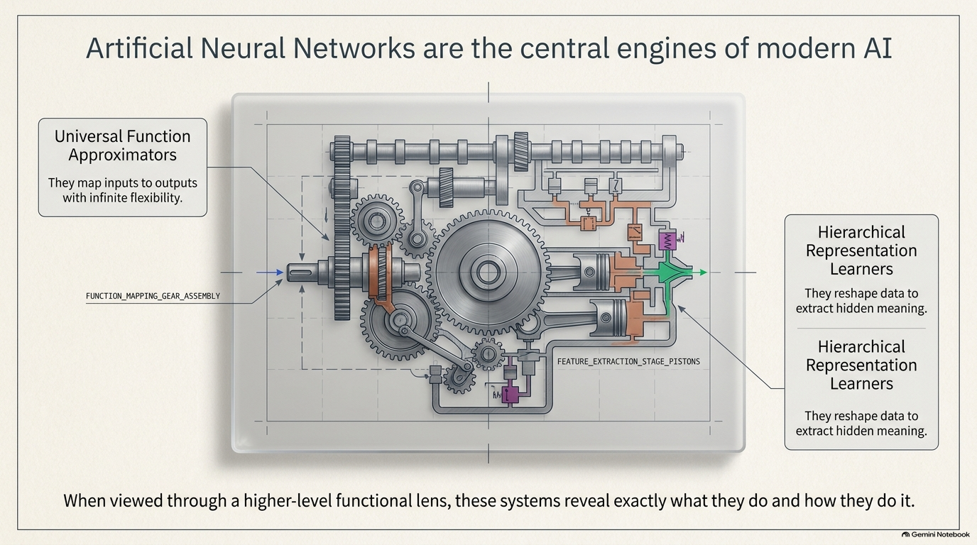
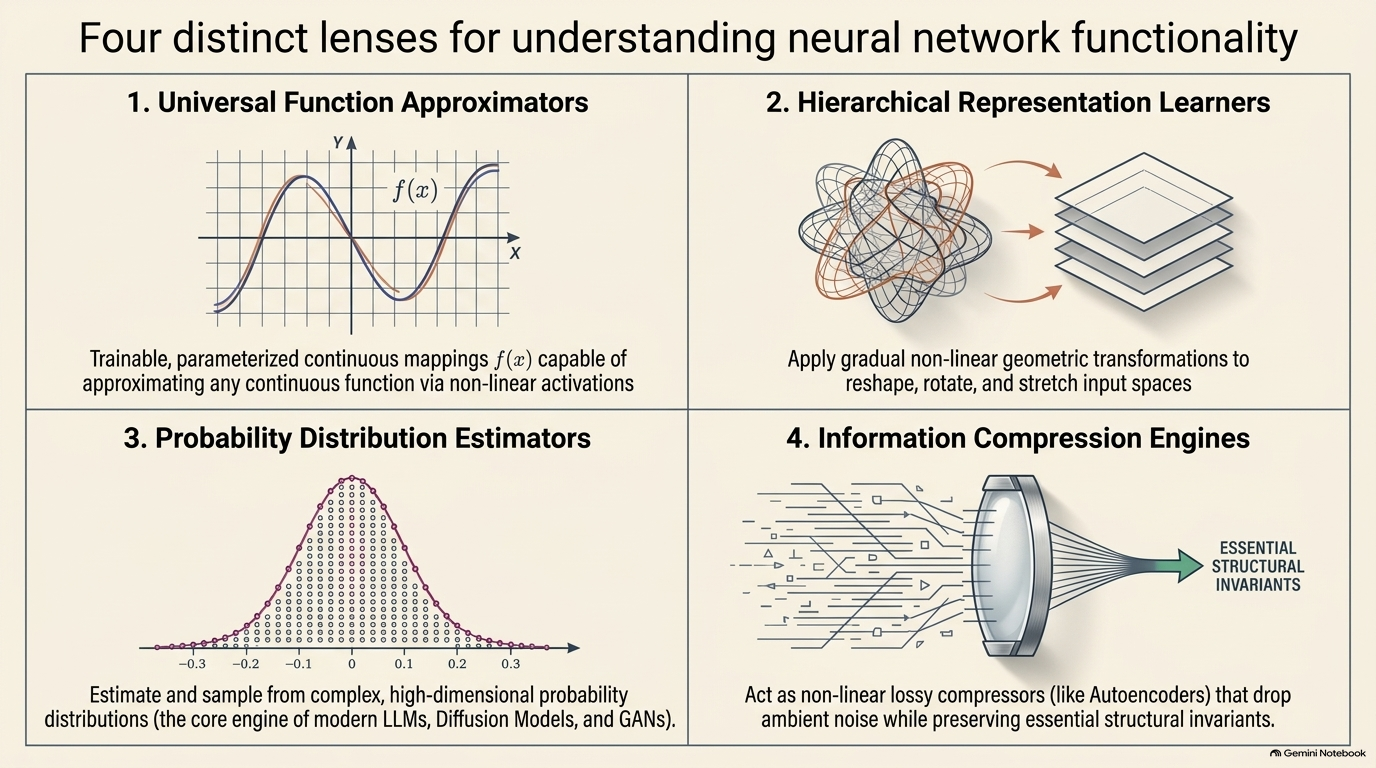
The same architecture, read four different ways depending on what the output is asked to represent.
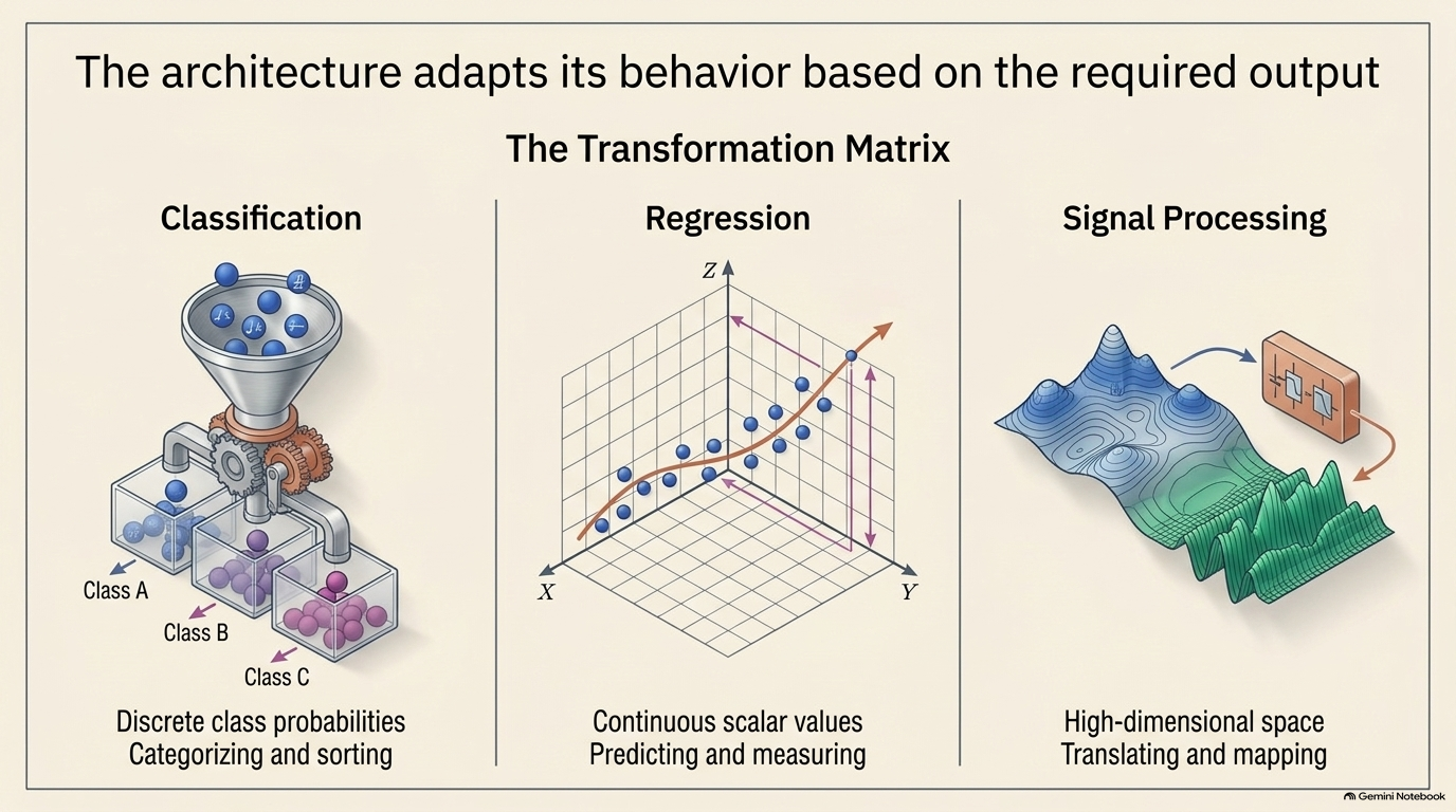
The same transformation matrix, pointed at three different jobs.
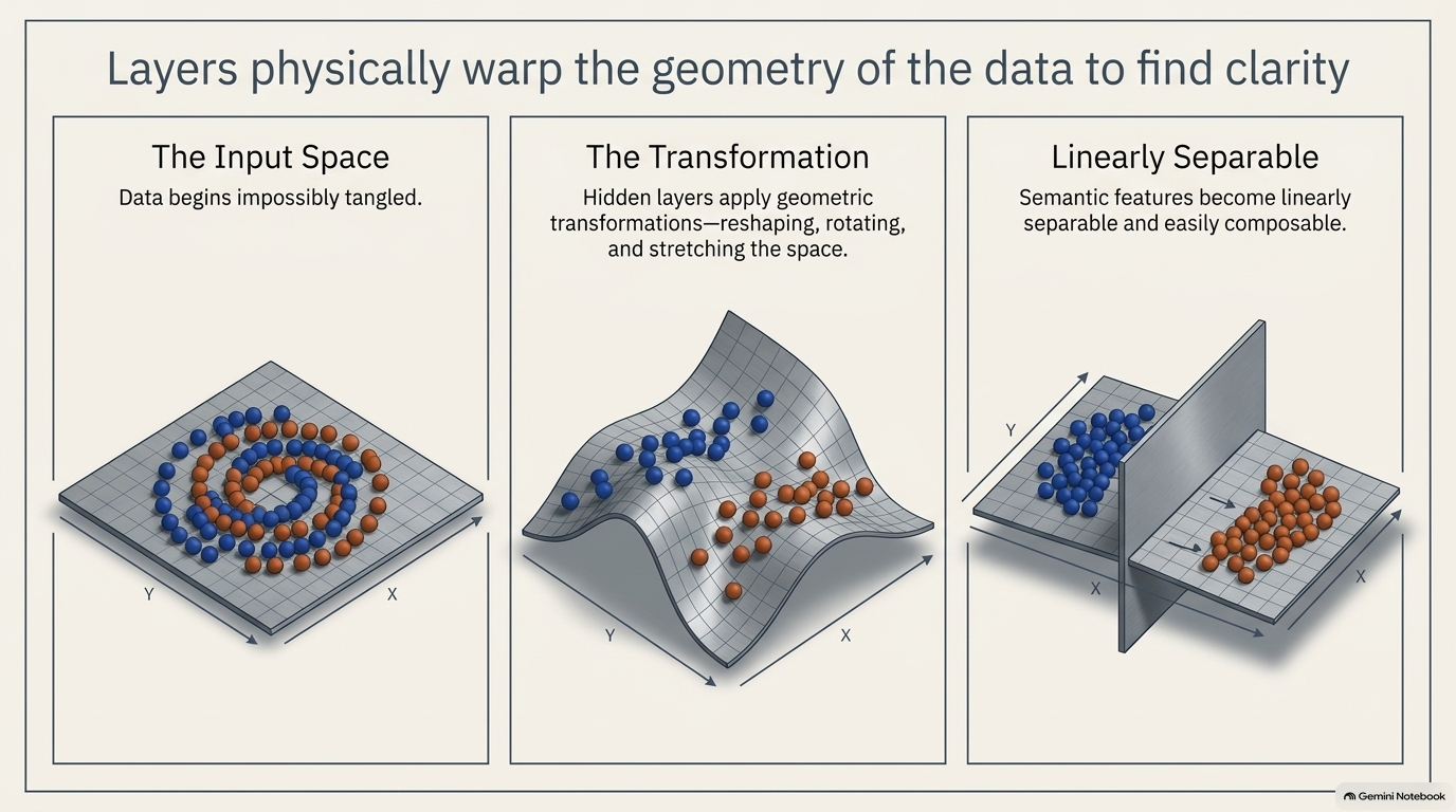
Hidden layers apply geometric transformations — reshaping, rotating, and stretching the space — until tangled classes become linearly separable.
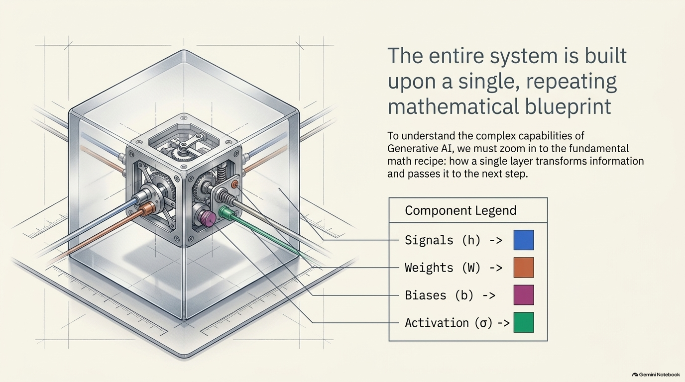
To understand the complex capabilities of generative AI, zoom in to the fundamental math recipe: how a single layer transforms information and passes it to the next step.
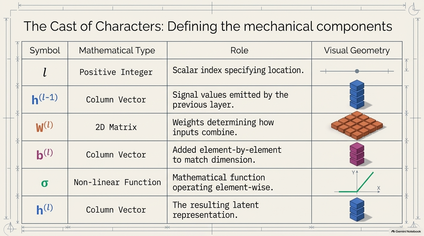
Every symbol in the layer equation, with its mathematical type and role.
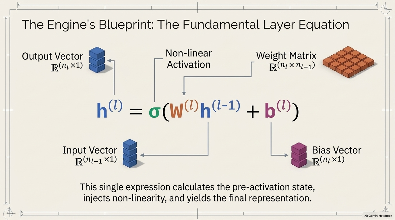
This single expression calculates the pre-activation state, injects non-linearity, and yields the final representation.
Every time a signal passes through a single layer of a neural network, it undergoes this exact sequential transformation.
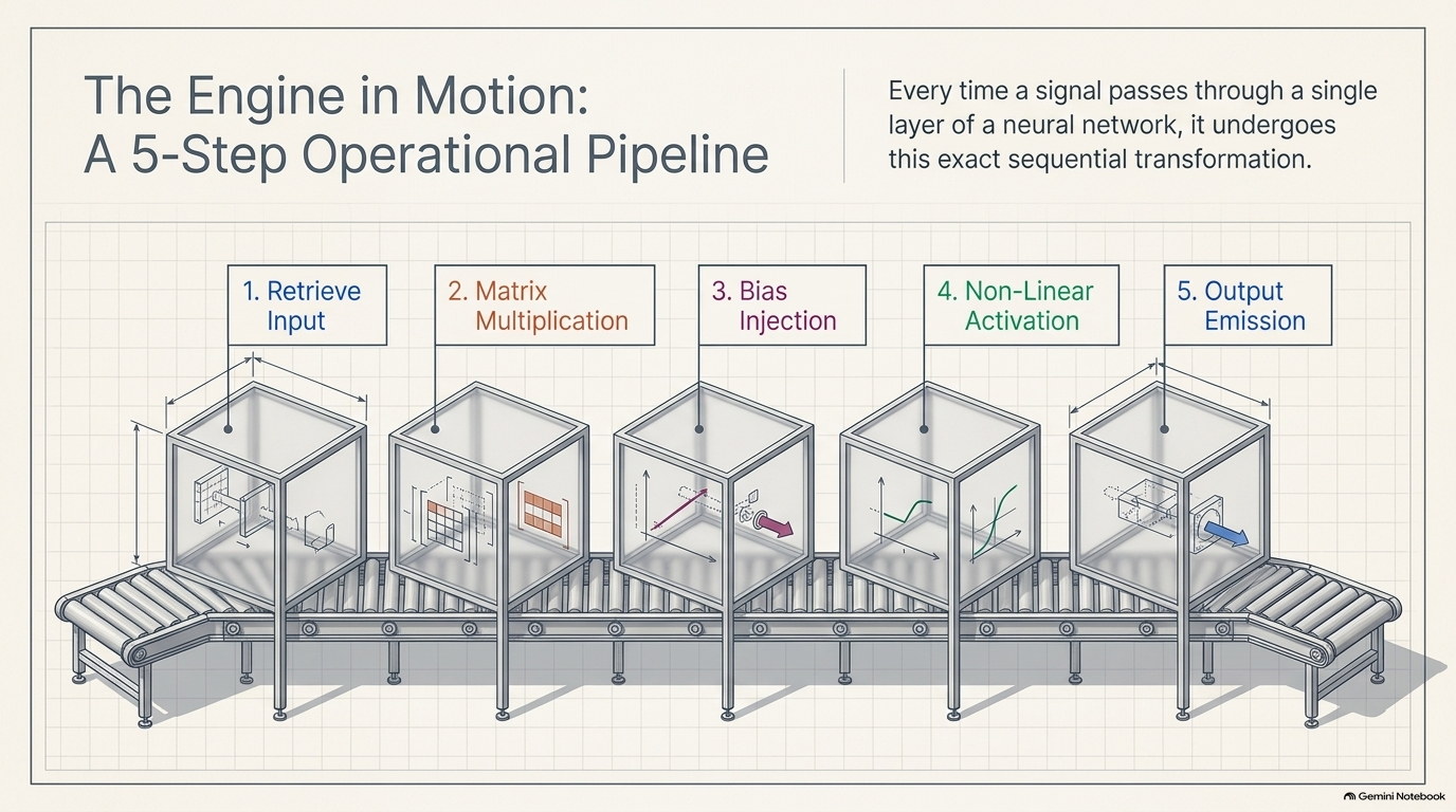
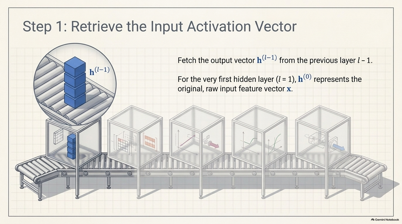
Fetch the output vector h(l−1) from the previous layer l−1.
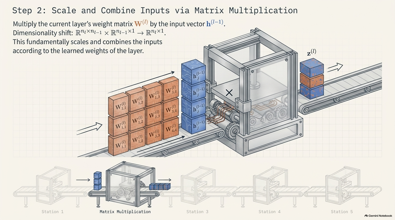
Multiply the current layer's weight matrix W(l) by the input vector h(l−1).
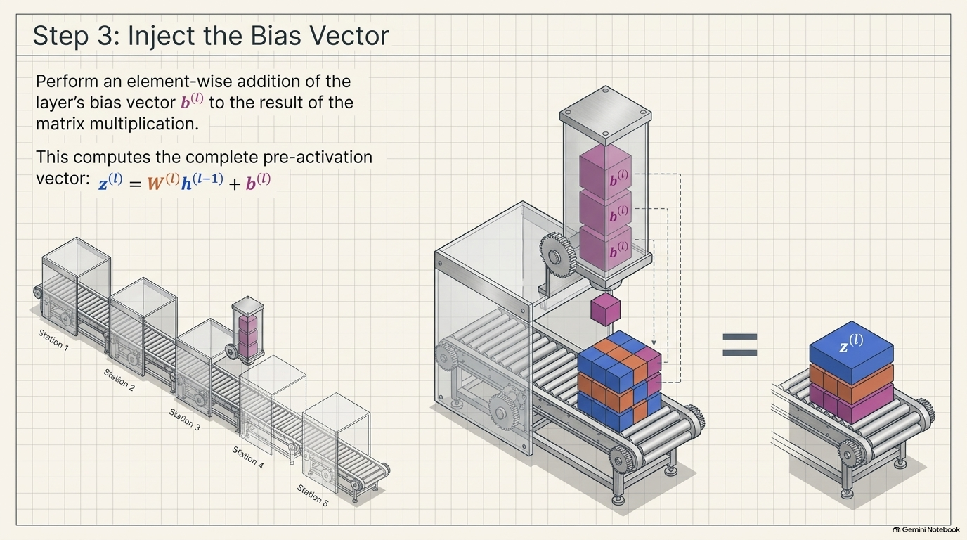
Perform an element-wise addition of the layer's bias vector b(l) to the result of the matrix multiplication.
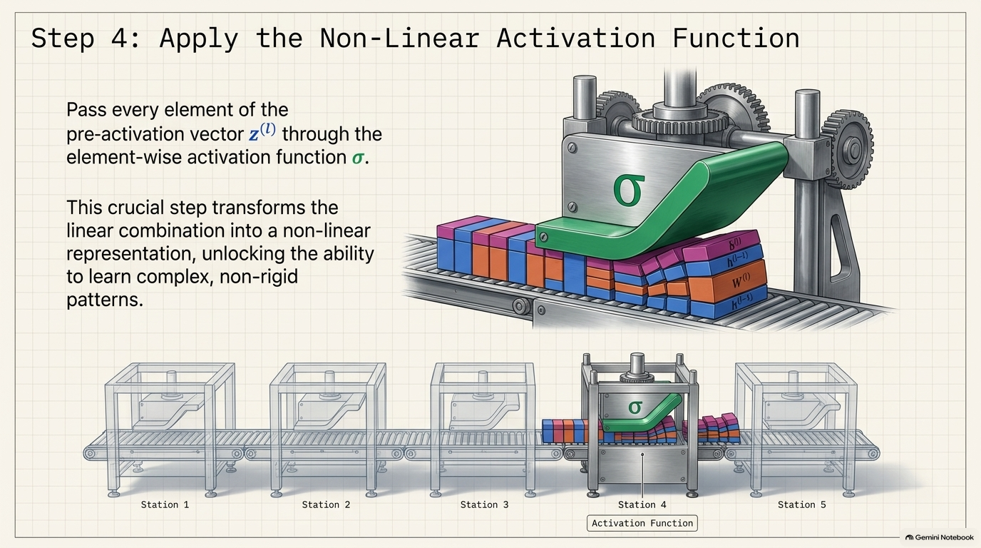
Pass every element of the pre-activation vector z(l) through the element-wise activation function σ.
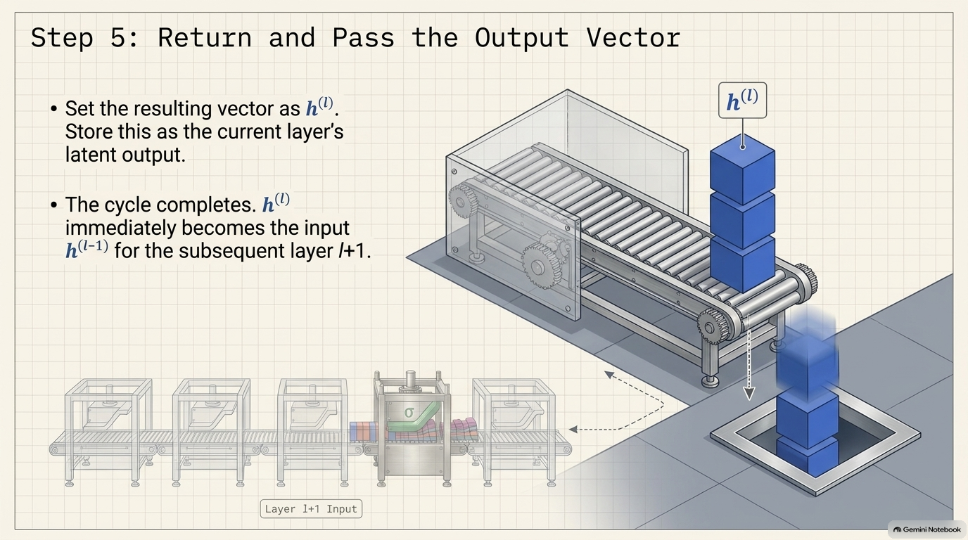
Set the resulting vector as h(l), and store it as the current layer's latent output.
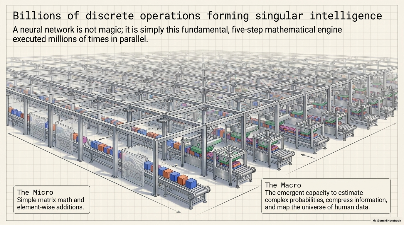
A neural network is not magic; it is simply this fundamental, five-step mathematical engine executed millions of times in parallel.
Artificial Neural Networks (ANNs) are the central component of modern AI. They function as a universal function approximator and a hierarchical representation learner — the same architecture read through four different functional lenses, and driven throughout by one small equation repeated at every layer.
1. Four ways to view what an ANN does
Universal Function Approximators. Mathematically, a neural network is a parameterized continuous mapping $f(x)$, where weights and biases are trainable. Per the Universal Approximation Theorem, a feedforward network with non-linear activation functions can approximate any continuous function. Classification occurs when the output represents discrete class probabilities; regression occurs when the output represents continuous scalar values; signal processing occurs when the output represents another high-dimensional space.
Hierarchical Representation Learners. Each hidden layer applies a non-linear geometric transformation. This process gradually reshapes, rotates, and stretches the input space until the underlying semantic features become linearly separable or easily composable.
Probability Distribution Estimators. In modern generative AI (LLMs, Diffusion Models, GANs), ANNs estimate and sample from complex, high-dimensional probability distributions.
Information Compression and Reconstruction Engines. Architectures like Autoencoders act as non-linear lossy compression engines. They learn to drop ambient noise while preserving the essential structural invariants, without assigning a class label.
2. The fundamental layer equation
This equation is the fundamental math recipe for how a single layer in a neural network transforms information and passes it to the next step: $$h^{(l)} = \sigma\!\left(W^{(l)} h^{(l-1)} + b^{(l)}\right)$$
| Symbol | Component name | Type | Dimensions | Role |
|---|---|---|---|---|
| $l$ | Layer index | Positive integer | $l \in \{1,2,\dots,L\}$ | A simple scalar index specifying location. |
| $h^{(l-1)}$ | Previous layer activation | Column vector | $\mathbb{R}^{n_{l-1}\times 1}$ | Signal values emitted by the previous layer. |
| $W^{(l)}$ | Weight matrix | 2D matrix | $\mathbb{R}^{n_l\times n_{l-1}}$ | Row $i$ holds the weights determining how all input features combine to influence neuron $i$. |
| $b^{(l)}$ | Bias vector | Column vector | $\mathbb{R}^{n_l\times 1}$ | Matches the output dimension, added element-by-element. |
| $\sigma$ | Activation function | Non-linear function | $\mathbb{R}\to\mathbb{R}$ | A mathematical function operating element-wise. |
| $h^{(l)}$ | Current layer output | Column vector | $\mathbb{R}^{n_l\times 1}$ | The resulting output vector — the network's latent representation at layer $l$. |
3. The five-step process
- Retrieve the input activation vector $h^{(l-1)}$. Fetch the output vector from the previous layer $l-1$. For the first hidden layer ($l=1$), $h^{(0)}$ represents the original input feature vector $x$.
- Perform matrix multiplication $W^{(l)}h^{(l-1)}$. Multiply the weight matrix $W^{(l)}$ of the current layer (dimensions $n_l\times n_{l-1}$) by the input vector $h^{(l-1)}$ (dimensions $n_{l-1}\times 1$). This scales and combines the inputs according to the layer's weights.
- Add the bias vector $b^{(l)}$. Perform an element-wise addition of the layer's bias vector $b^{(l)}$ (dimensions $n_l\times 1$) to the result of the matrix multiplication. This computes the pre-activation vector $z^{(l)} = W^{(l)}h^{(l-1)} + b^{(l)}$.
- Apply the non-linear activation function $\sigma$. Pass every element of the pre-activation vector $z^{(l)}$ through the element-wise activation function $\sigma$ (such as ReLU, Sigmoid, or Tanh). This transforms the linear combination into a non-linear representation.
- Return and pass the output vector $h^{(l)}$. Set the resulting activation vector as $h^{(l)}$ (dimensions $n_l\times 1$). Store $h^{(l)}$ as the current layer's output, which becomes the input $h^{(l-1)}$ for the next layer $l+1$.
Run millions of times in parallel across billions of these simple operations, this five-step engine is the entire mechanical basis for a neural network's capacity to estimate probabilities, compress information, and map the structure of real-world data.